Predict GRN from scRNA+scATAC data (Chen 2018 dataset)

Useful links:

Paper: https://www.biorxiv.org/content/10.1101/2023.06.09.543828v1

Github repo: https://github.com/cantinilab/HuMMuS

Documentation: https://cantinilab.github.io/HuMMuS/

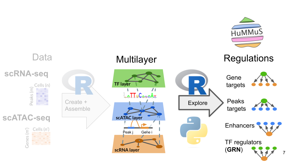
General description of the pipeline

Overall pipeline

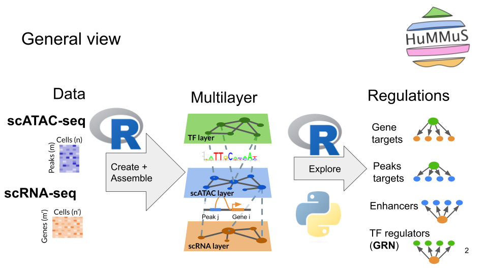
Useful ressources

Preprint detailing the method: https://www.biorxiv.org/content/10.1101/2023.06.09.543828v1

Github repo detailing the installation: https://github.com/cantinilab/HuMMuS

Documentation and vignette: https://cantinilab.github.io/HuMMuS

General plan

0. Preparation of the environment

1. Initialisation of a hummus object

2. Construction of the multilayer

3. Analyse multilayer and define gene regulatory network (GRN)

0. Setting up the environment

# install python dependency
envname = "r-reticulate"
# reticulate::py_install("hummuspy", envname = envname, pip=TRUE)
reticulate::use_condaenv(envname)

hummuspy <- reticulate::import("hummuspy")
library(HuMMuS)

##

Download the single-cell data

The data used in this tutorial can be downloaded here

1. Initialisation of HuMMuS object

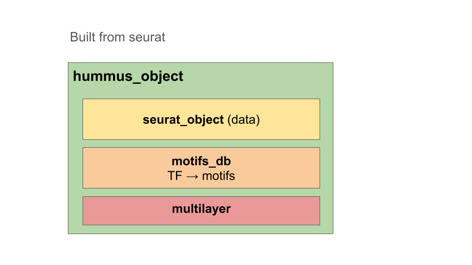
HuMMuS R objects are instances developed on top of seurat objects. It means it’s created from a seurat object and the contained assays can be accessed the same way.

Additionally, it contains a motifs_db object, providing tf motifs informations, and a multilayer objects, that will be completed while going through this tutorial. It will mostly include :

list of multiplex networks (one per modality)
list of bipartites (one per connection between layers)

1.1. Transform data into a hummus object

# Load the Chen dataset, which is a Seurat object containing scRNA-seq and scATAC-seq data
data("chen_dataset_subset")
chen_dataset_subset

## An object of class Seurat 
## 12000 features across 385 samples within 2 assays 
## Active assay: RNA (2000 features, 0 variable features)
##  2 layers present: counts, data
##  1 other assay present: peaks

# Create an hummus object from seurat object
hummus <- Initiate_Hummus_Object(chen_dataset_subset)

1.2. Add genome and motif annotations to hummus object

Fetch genome annotations online (necessitate an internet connection). You can also request any “EnsDB” object adapted to your data (e.g. EnsDb.Hsapiens.v86::EnsDb.Hsapiens.v86 for human genome annotations) or use your own genome annotations in the same format.

# get human genome annotation from EndDb data
# wrapper of Signac::GetGRangesFromEnsDb, adapting output to UCSC format
genome_annotations <- get_genome_annotations(
  ensdb_annotations = EnsDb.Hsapiens.v86::EnsDb.Hsapiens.v86)

# can also be downloaded, saved as an RDS objects for example

Add genome annotations to hummus/seurat object

Signac::Annotation(hummus@assays$peaks) <- genome_annotations
rm(genome_annotations)

Get TF motifs from JASPAR2020 and chromVARmotifs databsases in a motifs_db object. By default, human motifs are used. You can specify the species you want to use with the species argument (e.g. species = “mouse” for mouse). motifs_db objects contain 3 slots : * motifs = "PWMatrixList" * tf2motifs = "data.frame" * tfs = "NULL" PWMatrixList is a named vector of the motif matrices, whil tf2motifs is a correspondance table between TFs and motifs. tfs is a named vector of the TFs. You can also use your own motifs_db object, as long as it contains the same slots.

# Load TF motifs from JASPAR2020 and chromVARmotifs in hummus object
hummus@motifs_db <- get_tf2motifs() # by default human motifs

2. Construction of the multilayer

hummus object schema

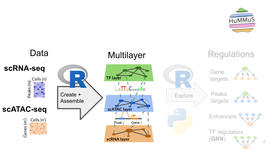
You can compute the different layers and bipartites as indicated below.

An example multilayer completed can also be imported with : data(chen_subset_hummus). This object corresponds to a multilayer from chen_dataset_subset completed. You can then go to the part 3, replacing hummus by chen_subset_hummus in each step.

Finally, you can compute the different layers before, and add them afterwards. It allows to use faster methods to compute the networks (e.g. Arboreto for the gene network, ATACNet for the peak network, etc.).

Compute 3 layers and 2 bipartites

hummus object schema

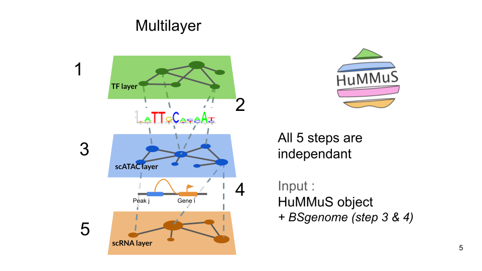
!! Long step !! You can also go directly to the part 3 for your “discovery tour”. :)

2.1. TF - peaks bipartite reconstruction

TF - peaks bipartite is computed using the motifs_db object and the peak assay. You can specify the assay to use to filter TFs (e.g. “RNA” if you want to use only the TFs expressed in your dataset). If NULL, all TFs with motifs will be used. BSGenome object is used to identify location of motifs and intersect them with peak
You can also specify the name of the bipartite that will be added to the hummus object. By default, it will be named “tf_peak”.

hummus <- bipartite_tfs2peaks(
              hummus_object = hummus,
              tf_expr_assay = "RNA", # use to filter TF on only expressed TFs,
                                     # if NULL, all TFs with motifs are used
              peak_assay = "peaks",
              tf_multiplex_name = "TF",
              genome = BSgenome.Hsapiens.UCSC.hg38::BSgenome.Hsapiens.UCSC.hg38,
              )

## Computing TF-peak bipartite
##   31 TFs expressed

## Building motif matrix

## Finding motif positions

## Creating Motif object

## Warning in CreateMotifObject(data = motif.matrix, positions = motif.positions,
## : Non-unique motif names supplied, making unique

##  Adding TF info
##  Returning TF-peak links as bipartite object
## no peak layer name provided, using peak_assay name

2.2. Genes - peaks bipartite reconstruction

Peaks - genes bipartite is computed

hummus <- bipartite_peaks2genes(
                      hummus_object = hummus,
                      gene_assay = "RNA",
                      peak_assay = "peaks",
                      store_network = FALSE,
                      )

Compute layer networks and add it to hummus object

Each one of the three layers is computed individually.

2.3. Compute the TF network from OmniPath database

We currently use OmniPath R package to fetch TF interactions. You can first specify if you want to use only the TFs expressed in your dataset (if you have a RNA assay in your hummus object). If gene_assay is NULL, all TFs with motifs will be used.
You can then specify which interactions you want to keep through ‘source_target’ argument (“AND” | “OR”). If “AND”, only the interactions between 2 TFs that are both present in the dataset will be kept. If “OR”, all interactions involving at least one TF present in the dataset will be kept.
Finally, you can specify the name of the multiplex and the name of the network that will be added to the hummus object. The added network will be undirected and unweighted since PPI and OmniPath database are not directional nor return any weight here.

hummus <- compute_tf_network(hummus,
                            gene_assay = "RNA", # default = None ;
                                                # If a assay is provided,
                                                # only the TFs that are present
                                                # will be considered
                            verbose = 1,
                            #source_target = "OR",
                            multiplex_name = "TF",
                            tf_network_name = "TF_network")

## Creating a fake TF network with all TFs connected to a fake node.
##   31 TFs expressed
## TF network construction time: 0.00711751 Creating new multiplex :  TF

2.4. Compute gene network from scRNA-seq w/ GENIE3

!! This step can be very slow if you have thousands of cells !!

Current recommendation if you have a big dataset is to compute the network before with GRNBoost2 thorugh arboreto and add it to the hummus object afterwards. Different methods can be used to compute the gene network. For now, only GENIE3 is implemented in HuMMuS. You can specify which assay to use to compute the network (gene_assay).
You can specify the number of cores to use to compute the network. You can also specify if you want to save the network locally (store_network = TRUE) or not (store_network = FALSE). If you choose to save the network, you will need to specify the output file name (output_file). The returned network will be considered undirected and weighted. While GENIE3 returns a directed network, we symmetrize it for the random walk with restart exploration of the genes proximity.

hummus <- compute_gene_network(
              hummus,
              gene_assay = "RNA",
              method = "GENIE3",
              verbose = 1,
              number_cores = 5, # GENIE3 method can be ran
                                # parallelised on multiple cores
              store_network = FALSE, # by default : FALSE, but
                                     # each network can be saved 
                                     # when computed with hummus
              output_file = "gene_network.tsv")

## Computing gene network with  GENIE3  ...
##  No TFs list provided, fetching from hummus object...
##   31 TFs expressed
##  Gene network construction time: 7.689511 
##  Creating new multiplex :  RNA

2.5. Compute the peak network from scATAC-seq w/ Cicero

Different methods can be used to compute the peak network. For now, only Cicero is implemented in HuMMuS. You can specify which assay to use to compute the network (peak_assay). You can also specify the number of cores to use to compute the network. You can also specify if you want to save the network locally (store_network = TRUE) or not (store_network = FALSE). If you choose to save the network, you will need to specify the output file name (output_file). The returned network will be considered undirected and weighted, since cis-regulatory interaction and Cicero outputs are not directional.

hummus <- compute_atac_peak_network(hummus,
              atac_assay = "peaks",
              verbose = 1,
              genome = BSgenome.Hsapiens.UCSC.hg38::BSgenome.Hsapiens.UCSC.hg38,
              store_network = FALSE)

## Overlap QC metrics:
## Cells per bin: 50
## Maximum shared cells bin-bin: 44
## Mean shared cells bin-bin: 6.39503105590062
## Median shared cells bin-bin: 0

## Warning in cicero::make_cicero_cds(input_cds, reduced_coordinates =
## umap_coords, : On average, more than 10% of cells are shared between paired
## bins.

## [1] "Starting Cicero"
## [1] "Calculating distance_parameter value"

## Warning in estimate_distance_parameter(cds, window = window, maxit = 100, :
## Could not calculate sample_num distance_parameters (74 were calculated) - see
## documentation details

## [1] "Running models"
## [1] "Assembling connections"
## [1] "Successful cicero models:  4782"
## [1] "Other models: "
## 
## Zero or one element in range 
##                         8803 
## [1] "Models with errors:  0"
## [1] "Done"
## 
##  4793 peak edges with a coaccess score > 0 were found.
## Peak network construction time: 27.22618 Creating new multiplex :  peaks

3. Analyse of the multilayer and definition of GRN

data(chen_subset_hummus) 
hummus <- chen_subset_hummus

3.1. Save the mulilayer in a classic hierarchical structure

The package used for the random walk with restart exploration (multixrank) requires currently to save all the network files on disk. To simplify the organisation of the file, it is possible to save everything necessary with function save_multilayer().
It will create a folder (specified through folder_name) containing all the files necessary to run the multixrank algorithm. The folder will contain the following subfolders : * bipartite : containing the bipartites files * multiplex : containing the multiplex sub-subfolders * multiplex_1 (e.g. TF|peak|RNA) : containing the network file of each layer of the multiplex * seed : that will contain the seed files (necessary to compute HuMMuS outputs later) * config : that will contain the config files (necessary to compute HuMMuS outputs later)

hummus object schema

save_multilayer(hummus = hummus,
                folder_name = "chen_multilayer")

## Warning in dir.create(folder_name): 'chen_multilayer' already exists

## Warning in dir.create(paste0(folder_name, "/", multiplex_folder)):
## 'chen_multilayer/multiplex' already exists

## Warning in dir.create(paste0(folder_name, "/", bipartite_folder)):
## 'chen_multilayer/bipartite' already exists

## Multiplex of  1  networks with 32 features.
##  Networks names:  TF_network[1] "TF TF_network"

## Warning in dir.create(paste0(folder_name, "/", multiplex_folder, "/",
## multiplex_name)): 'chen_multilayer/multiplex/RNA' already exists

## Multiplex of  1  networks with 2000 features.
##  Networks names:  RNA_GENIE3[1] "RNA RNA_GENIE3"
## Multiplex of  1  networks with 4639 features.
##  Networks names:  peak_network_cicero[1] "peaks peak_network_cicero"

3.2. Retrieve target genes

With HuMMuS, inference of GRN and target gene of TFs are different outputs. Indeed, while GRN is computed making TFs compete to regulate genes (by random walk with restart starting from the genes and going to the TFs), target genes are computed making genes compete to be regulated by TFs (by random walk with restart starting from the TFs and going to the genes).
For target genes output, you can specify the list of TFs (tf_list) to use as seed (if NULL by default, all TFs will be used as seed). Only the links between the seed TFs and the genes will be computed. You can also specify the list of genes to use. Only the score of the genes present in the network and the gene_list will be returned.

ATF2_genes <- define_target_genes(
  hummus,
  tf_list = list("ATF2"),
  multilayer_f = "chen_multilayer",
  njobs = 1
  )

## multiplexes_list :  {'TF': {'TF_network': '00'}, 'RNA': {'RNA_GENIE3': '01'}, 'peaks': {'peak_network_cicero': '01'}}
## bipartites_list :  {'tf_peak.tsv': {'multiplex_right': 'TF', 'multiplex_left': 'peaks'}, 'atac_rna.tsv': {'multiplex_right': 'peaks', 'multiplex_left': 'RNA'}}
## folder_multiplexes :  multiplex
## folder_bipartites :  bipartite
## gene_list :  None
## tf_list :  ['ATF2']
## peak_list :  None
## config_filename :  target_genes_config.yml
## config_folder :  config
## tf_multiplex :  TF
## peak_multiplex :  peaks
## rna_multiplex :  RNA
## update_config :  True
## save :  False
## return_df :  True
## output_f :  None
## njobs :  1
## {'TF': {'TF_network': '00'}, 'RNA': {'RNA_GENIE3': '01'}, 'peaks': {'peak_network_cicero': '01'}}
## bipartites_type has been provided throguh a list, make sure the order matches the one of the 'bipartites' dictionary' keys.
## {'RNA': {'names': ['RNA_1'], 'graph_type': ['01'], 'layers': ['chen_multilayer/multiplex/RNA/RNA_GENIE3.tsv']}, 'TF': {'names': ['TF_1'], 'graph_type': ['00'], 'layers': ['chen_multilayer/multiplex/TF/TF_network.tsv']}, 'peaks': {'names': ['peaks_1'], 'graph_type': ['01'], 'layers': ['chen_multilayer/multiplex/peaks/peak_network_cicero.tsv']}}
## ('RNA_1',)
## RNA_1
## Opening network from chen_multilayer/multiplex/RNA/RNA_GENIE3.tsv.
## ('TF_1',)
## TF_1
## Opening network from chen_multilayer/multiplex/TF/TF_network.tsv.
## ('peaks_1',)
## peaks_1
## Opening network from chen_multilayer/multiplex/peaks/peak_network_cicero.tsv.
## {'source': 'peaks', 'target': 'TF', 'graph_type': '00', 'edge_list_df': 'chen_multilayer/bipartite/tf_peak.tsv'}
## Opening network from chen_multilayer/bipartite/tf_peak.tsv.
## {'source': 'RNA', 'target': 'peaks', 'graph_type': '00', 'edge_list_df': 'chen_multilayer/bipartite/atac_rna.tsv'}
## Opening network from chen_multilayer/bipartite/atac_rna.tsv.
## 1
## http://127.0.0.1:8787/status
## Processing seeds... ━━━━━━━━━━━━━━━━━━━━━━━━━━━━━━━━━━━━━━━━ 100% 0:00:00

head(ATF2_genes)

##   index layer path_layer        score   tf     gene
## 1  1175   RNA      RNA_1 5.291440e-05 ATF2    CDC5L
## 2   540   RNA      RNA_1 4.570328e-05 ATF2     ATF3
## 3   591   RNA      RNA_1 4.486208e-05 ATF2    ATP5I
## 4  1096   RNA      RNA_1 4.485191e-05 ATF2 CCNB1IP1
## 5  1872   RNA      RNA_1 4.482241e-05 ATF2   DGCR14
## 6   536   RNA      RNA_1 4.176609e-05 ATF2    ATAT1

target_genes <- define_target_genes(
  hummus,
  multilayer_f = "chen_multilayer",
  njobs = 1
  )

## multiplexes_list :  {'TF': {'TF_network': '00'}, 'RNA': {'RNA_GENIE3': '01'}, 'peaks': {'peak_network_cicero': '01'}}
## bipartites_list :  {'tf_peak.tsv': {'multiplex_right': 'TF', 'multiplex_left': 'peaks'}, 'atac_rna.tsv': {'multiplex_right': 'peaks', 'multiplex_left': 'RNA'}}
## folder_multiplexes :  multiplex
## folder_bipartites :  bipartite
## gene_list :  None
## tf_list :  None
## peak_list :  None
## config_filename :  target_genes_config.yml
## config_folder :  config
## tf_multiplex :  TF
## peak_multiplex :  peaks
## rna_multiplex :  RNA
## update_config :  True
## save :  False
## return_df :  True
## output_f :  None
## njobs :  1
## {'TF': {'TF_network': '00'}, 'RNA': {'RNA_GENIE3': '01'}, 'peaks': {'peak_network_cicero': '01'}}
## bipartites_type has been provided throguh a list, make sure the order matches the one of the 'bipartites' dictionary' keys.
## {'RNA': {'names': ['RNA_1'], 'graph_type': ['01'], 'layers': ['chen_multilayer/multiplex/RNA/RNA_GENIE3.tsv']}, 'TF': {'names': ['TF_1'], 'graph_type': ['00'], 'layers': ['chen_multilayer/multiplex/TF/TF_network.tsv']}, 'peaks': {'names': ['peaks_1'], 'graph_type': ['01'], 'layers': ['chen_multilayer/multiplex/peaks/peak_network_cicero.tsv']}}
## ('RNA_1',)
## RNA_1
## Opening network from chen_multilayer/multiplex/RNA/RNA_GENIE3.tsv.
## ('TF_1',)
## TF_1
## Opening network from chen_multilayer/multiplex/TF/TF_network.tsv.
## ('peaks_1',)
## peaks_1
## Opening network from chen_multilayer/multiplex/peaks/peak_network_cicero.tsv.
## {'source': 'peaks', 'target': 'TF', 'graph_type': '00', 'edge_list_df': 'chen_multilayer/bipartite/tf_peak.tsv'}
## Opening network from chen_multilayer/bipartite/tf_peak.tsv.
## {'source': 'RNA', 'target': 'peaks', 'graph_type': '00', 'edge_list_df': 'chen_multilayer/bipartite/atac_rna.tsv'}
## Opening network from chen_multilayer/bipartite/atac_rna.tsv.
## 31
## http://127.0.0.1:8787/status
## Processing seeds... ━━━━━━━━━━━━━━━━━━━━━━━━━━━━━━━━━━━━━━━━ 100% 0:00:00

head(target_genes)

##   index layer path_layer        score   tf     gene
## 1  1340   RNA      RNA_1 0.0002318541 CUX1   CHRNB1
## 2  1175   RNA      RNA_1 0.0002299783 CUX1    CDC5L
## 3   262   RNA      RNA_1 0.0002217501 CUX1    ALG11
## 4  1182   RNA      RNA_1 0.0002211187 CUX1    CDCA5
## 5   196   RNA      RNA_1 0.0002201921 CUX1    AGBL5
## 6  1172   RNA      RNA_1 0.0001498125 BPTF CDC42SE1

3.3. Define GRN

The GRN is defined using the multixrank algorithm. It requires to have the hummuspy python package installed (pip install hummuspy).

This can be parallelised using the njobs argument. You can also specify the list of genes and the list of TFs to use.

grn <- define_grn(
  hummus,
  multilayer_f = "chen_multilayer",
  njobs = 5
  )

grn

3.4. Retrieve enhancers

You can also specify the list of peaks to use.

enhancers <- define_enhancers(
  hummus,
  gene_list = list("ATF2"),
  multilayer_f = "chen_multilayer",
  njobs = 1
  )

## multiplexes_list :  {'TF': {'TF_network': '00'}, 'RNA': {'RNA_GENIE3': '01'}, 'peaks': {'peak_network_cicero': '01'}}
## bipartites_list :  {'tf_peak.tsv': {'multiplex_right': 'TF', 'multiplex_left': 'peaks'}, 'atac_rna.tsv': {'multiplex_right': 'peaks', 'multiplex_left': 'RNA'}}
## folder_multiplexes :  multiplex
## folder_bipartites :  bipartite
## gene_list :  ['ATF2']
## tf_list :  None
## peak_list :  None
## config_filename :  enhancers_config.yml
## config_folder :  config
## tf_multiplex :  TF
## peak_multiplex :  peaks
## rna_multiplex :  RNA
## update_config :  True
## save :  False
## return_df :  True
## output_f :  None
## njobs :  1
## {'TF': {'TF_network': '00'}, 'RNA': {'RNA_GENIE3': '01'}, 'peaks': {'peak_network_cicero': '01'}}
## bipartites_type has been provided throguh a list, make sure the order matches the one of the 'bipartites' dictionary' keys.
## {'RNA': {'names': ['RNA_1'], 'graph_type': ['01'], 'layers': ['chen_multilayer/multiplex/RNA/RNA_GENIE3.tsv']}, 'TF': {'names': ['TF_1'], 'graph_type': ['00'], 'layers': ['chen_multilayer/multiplex/TF/TF_network.tsv']}, 'peaks': {'names': ['peaks_1'], 'graph_type': ['01'], 'layers': ['chen_multilayer/multiplex/peaks/peak_network_cicero.tsv']}}
## ('RNA_1',)
## RNA_1
## Opening network from chen_multilayer/multiplex/RNA/RNA_GENIE3.tsv.
## ('TF_1',)
## TF_1
## Opening network from chen_multilayer/multiplex/TF/TF_network.tsv.
## ('peaks_1',)
## peaks_1
## Opening network from chen_multilayer/multiplex/peaks/peak_network_cicero.tsv.
## {'source': 'peaks', 'target': 'TF', 'graph_type': '00', 'edge_list_df': 'chen_multilayer/bipartite/tf_peak.tsv'}
## Opening network from chen_multilayer/bipartite/tf_peak.tsv.
## {'source': 'RNA', 'target': 'peaks', 'graph_type': '00', 'edge_list_df': 'chen_multilayer/bipartite/atac_rna.tsv'}
## Opening network from chen_multilayer/bipartite/atac_rna.tsv.
## 1
## http://127.0.0.1:8787/status
## Processing seeds... ━━━━━━━━━━━━━━━━━━━━━━━━━━━━━━━━━━━━━━━━ 100% 0:00:00

head(enhancers)

##   index layer path_layer        score gene                     peak
## 1  3950 peaks    peaks_1 0.0008951819 ATF2   chr6-44387360-44388305
## 2  3134 peaks    peaks_1 0.0007383304 ATF2 chr3-107522766-107524070
## 3  4007 peaks    peaks_1 0.0006763254 ATF2 chr7-102125135-102125606
## 4  4189 peaks    peaks_1 0.0004115710 ATF2   chr7-73738654-73739271
## 5   676 peaks    peaks_1 0.0003972408 ATF2  chr10-73874242-73875104
## 6  1699 peaks    peaks_1 0.0003850920 ATF2  chr16-67561885-67563510

3.5. Retrieve binding regions

For binding regions output, you can specify the list of TFs (tf_list) to use as seed (if NULL by default, all TFs will be used as seed). Only the links between the seed TFs and the peaks will be computed. You can also specify the list of peaks to use. Only the score of the peaks present in the network and the peak_list will be returned.

binding_regions <- define_binding_regions(
  hummus,
  multilayer_f = "chen_multilayer",
  njobs = 1
  )

## multiplexes_list :  {'TF': {'TF_network': '00'}, 'RNA': {'RNA_GENIE3': '01'}, 'peaks': {'peak_network_cicero': '01'}}
## bipartites_list :  {'tf_peak.tsv': {'multiplex_right': 'TF', 'multiplex_left': 'peaks'}, 'atac_rna.tsv': {'multiplex_right': 'peaks', 'multiplex_left': 'RNA'}}
## folder_multiplexes :  multiplex
## folder_bipartites :  bipartite
## gene_list :  None
## tf_list :  None
## peak_list :  None
## config_filename :  binding_regions_config.yml
## config_folder :  config
## tf_multiplex :  TF
## peak_multiplex :  peaks
## rna_multiplex :  RNA
## update_config :  True
## save :  False
## return_df :  True
## output_f :  None
## njobs :  1
## {'TF': {'TF_network': '00'}, 'RNA': {'RNA_GENIE3': '01'}, 'peaks': {'peak_network_cicero': '01'}}
## bipartites_type has been provided throguh a list, make sure the order matches the one of the 'bipartites' dictionary' keys.
## {'RNA': {'names': ['RNA_1'], 'graph_type': ['01'], 'layers': ['chen_multilayer/multiplex/RNA/RNA_GENIE3.tsv']}, 'TF': {'names': ['TF_1'], 'graph_type': ['00'], 'layers': ['chen_multilayer/multiplex/TF/TF_network.tsv']}, 'peaks': {'names': ['peaks_1'], 'graph_type': ['01'], 'layers': ['chen_multilayer/multiplex/peaks/peak_network_cicero.tsv']}}
## ('RNA_1',)
## RNA_1
## Opening network from chen_multilayer/multiplex/RNA/RNA_GENIE3.tsv.
## ('TF_1',)
## TF_1
## Opening network from chen_multilayer/multiplex/TF/TF_network.tsv.
## ('peaks_1',)
## peaks_1
## Opening network from chen_multilayer/multiplex/peaks/peak_network_cicero.tsv.
## {'source': 'peaks', 'target': 'TF', 'graph_type': '00', 'edge_list_df': 'chen_multilayer/bipartite/tf_peak.tsv'}
## Opening network from chen_multilayer/bipartite/tf_peak.tsv.
## {'source': 'RNA', 'target': 'peaks', 'graph_type': '00', 'edge_list_df': 'chen_multilayer/bipartite/atac_rna.tsv'}
## Opening network from chen_multilayer/bipartite/atac_rna.tsv.
## 31
## http://127.0.0.1:8787/status
## Processing seeds... ━━━━━━━━━━━━━━━━━━━━━━━━━━━━━━━━━━━━━━━━ 100% 0:00:00

head(binding_regions)

##   index layer path_layer       score   tf                     peak
## 1   464 peaks    peaks_1 0.001680402 CUX1   chr1-65002512-65003322
## 2  4617 peaks    peaks_1 0.001675393 CUX1   chrX-48971714-48972653
## 3   468 peaks    peaks_1 0.001674121 CUX1   chr1-65419692-65420979
## 4  4615 peaks    peaks_1 0.001559648 CUX1   chrX-48918888-48919598
## 5  4307 peaks    peaks_1 0.001502478 CUX1   chr8-24955892-24956818
## 6  2655 peaks    peaks_1 0.001502093 CUX1 chr2-201642365-201643651

Trimbour Rémi

2023-05-16

Useful links:

General description of the pipeline

Useful ressources

General plan

0. Preparation of the environment

1. Initialisation of a hummus object

2. Construction of the multilayer

3. Analyse multilayer and define gene regulatory network (GRN)

0. Setting up the environment

Download the single-cell data

1. Initialisation of HuMMuS object

1.1. Transform data into a hummus object

1.2. Add genome and motif annotations to hummus object

2. Construction of the multilayer

Compute 3 layers and 2 bipartites

2.1. TF - peaks bipartite reconstruction

2.2. Genes - peaks bipartite reconstruction

Compute layer networks and add it to hummus object

2.3. Compute the TF network from OmniPath database

2.4. Compute gene network from scRNA-seq w/ GENIE3

!! This step can be very slow if you have thousands of cells !!

2.5. Compute the peak network from scATAC-seq w/ Cicero

3. Analyse of the multilayer and definition of GRN

3.1. Save the mulilayer in a classic hierarchical structure

3.2. Retrieve target genes

3.3. Define GRN

3.4. Retrieve enhancers

3.5. Retrieve binding regions